Words Alone: Dismantling Topic Models in the Humanities
Benjamin M. Schmidt
As this issue shows, there is no shortage of interest among humanists in using topic modeling. An entire genre of introductory posts has emerged encouraging humanists to try LDA.[1] So many scholars in humanities departments are turning to the tool in their research that it is sometimes described as part of the digital humanities in itself. Last fall, the NEH sponsored a workshop at Maryland which expressed concern that “the most promising work in topic modeling is being done not by humanists exploring literary or historical corpora but instead by scholars working in natural language processing and information retrieval.” There is not, it seems safe to say, another machine-learning algorithm in the world anyone would expect humanists to lead the progress of. Newcomers to the field could be forgiven for thinking that digital humanists need to topic model to prove their mettle; analog humanists could be forgiven for assuming that the computational interests of literary scholars and historians are particularly focused on the sorts of questions that topic models answer.
As all these scholars have said, the technique has a number of promising applications in the humanities. It does a good job giving an overview of the contents of large textual collections; it can provide some intriguing new artifacts to study; and it even holds, as I will show below, some promise for structuring non-lexical data like geographic points. But simplifying topic models for humanists who will not (and should not) study the underlying algorithms creates an enormous potential for groundless — or even misleading — “insights.”
Much of the apparent ease and intuitiveness of topic models comes from a set of assumptions that are only partially true. To make topic models present new raw material for humanists to read, analysts generally assume that an individual topic produced by the algorithm has two properties. First, it is coherent: a topic is a set of words that all tend to appear together, and will therefore have a number of things in common. Second, it is stable: if a topic appears at the same rate in two different types of documents, it means essentially the same thing in both. Together, these let humanists assume that the co-occurrence patterns described by topics are meaningful; topics are useful because they describe things that resemble “concepts,” “discourses,” or “fields.”
When these assumptions hold, topics offer an immense improvement over studying individual words to understand massive text corpora. Words are frustrating entities to study. Although higher order entities like concepts are all ultimately constituted through words, no word or group can easily stand in for any of them. The appeal of topic modeling for many humanists is that it makes it possible to effortlessly and objectively create aggregates that seem to be more meaningful than the words that constitute them.
But topics neither can nor should be studied independently of a deep engagement in the actual word counts that build them. Like words, they are messy, ambiguous, and elusive. When humanists examine the output from MALLET (the most widely used topic-modeling tool), they need to be aware of the ways that topics may not be as coherent as they assume. The predominant practice among humanists using topic modeling ensures that they will never see the ways their assumptions fail them. To avoid being misled by all the excitement, humanists need to ground the analysis of topic models in the words they are built from. From lifelong experience, humanists know how words can mislead us. They do not know how topics fail our assumptions.
This article suggests two ways to bring words back to topic models in humanistic practice, which destabilizes some of the assumptions that make topic models so appealing. The first, using geographical data, shows the problems with labeling topics based on the top five to ten words and the ways that assumptions of meaningfulness and coherence are not grounded. The second shows the dangers of accepting a topic model’s assumption of topic stability across different sorts of documents: extremely common practices, such as plotting topic frequencies across time, can elide dramatic differences in what words different documents actually use. In both cases, visualization that uses the individual word assignments, not just the topic labels, can help dramatically change the readings that humanists give to topics.
New ways of reading the composition of topics are necessary, because humanists seem to want to do slightly different things with topic models than the computer scientists who invented them and know them best. Latent Direchlet Allocation (so widely used as a topic modeling algorithm that I will use “LDA” interchangeably with the general term here) was first described by David Blei et al in 2003.[2] Blei’s group at Princeton most often describes LDA as an advance in information retrieval. It can make, Blei shows, large collections of text browsable by giving useful tags to the documents. (Some of Blei’s uses are here and here; Jonathan Goodwin has recently adapted a similar model for JSTOR articles in rhetoric and literary theory.) When confronted with a massive store of unstructured documents, topic models let you “read” the topic headings first, and then only search out articles in the topics that interest you. Much like traditional library subject headings, topic models let you search for the intersection of two related fields, can help bring new documents to your attention, and give a sense of the dominant themes in a library.
For these purposes, meaningful labels are incredibly important, and occasional misfilings unimportant. (If a document is “misfiled” into the wrong topic, the researcher simply will skip over it). But while topic models can be immensely powerful for browsing and isolating results in thousands or millions of uncatalogued texts, scholars in literature and history working with text usually have extensive data about the documents they have. A standard citation includes not just an author but a date, a city, and a publisher. Unstructured browsing is rarely useful: the interactions among metadata fields are at the heart of the researcher’s interest.
Humanists seem to be using topic models, instead, for “discovery” in quite a different sense. Topic compositions, and the labels they receive, are taken as something that might generate new perspectives on texts. As Trevor Owens describes it, “anything goes in the generative world of discovery.” Topic modeling enables a process of reconfigurations that can lead humanists to new insights. In this frame, topic models are only as useful or as problematic as those who use them say they are.
Still, excitement about the use of topic models for discovery needs to be tempered with skepticism about how often the unexpected juxtapositions LDA creates will be helpful, and how often merely surprising. A poorly supervised machine learning algorithm is like a bad research assistant. It might produce some unexpected constellations that show flickers of deeper truths; but it will also produce tedious, inexplicable, or misleading results. If it is not doing the desired task, it is time to give it some clearer instructions, or to find a new one. Much of the excitement over topic models is that they seem to work better than other rearrangement algorithms.
It is even possible to imagine a sort of “placebo” effect of topic modeling. By giving humanists the feeling that they are exploring large corpora much more quickly and efficiently at scale, topic models may make humanists much more willing to entertain big-picture questions about huge textual libraries. Historians and literature scholars might be able to start to tackle questions spanning centuries and tens of thousands of texts through more traditional means, using topic models only to make the initial process of venturing new ideas feel less unbounded. Confidence gained in this manner may be quite useful. But it remains important to know the ways that the tool might not be working.
Topic Modeling at Sea
The idea that topics are meaningful rests, in large part, on assumptions of their coherence derived from checking the list of the most frequent words. But the top few words in a topic only give a small sense of the thousands of the words that constitute the whole probability distribution. In order to get a sense of what it might look like to analyze all the words in a topic at once, we can turn to topic models applied to data that are not, in the conventional sense, words at all. Topic models, fundamentally, are clustering algorithms that create groupings based on the distributional properties of words across documents. The distributional patterns that words show, however, are not particularly special: all sorts of other datasets show similar properties. In computer science, LDA is used for many kinds of non-textual data, from images to music.
I have been looking for some time at digitized ships’ logs, in part as an arena to think about problems in reading digital texts. Ships’ logs are ideal candidates for machine learning algorithms — like texts, they contained large amounts of partially structured data. A logbook is, after all, a book that has been simply been digitized to an extremely rigid vocabulary of points in space and time. Hundreds of thousands of ships’ voyages have been digitized by climatologists. (Here, I am looking at some of the oldest voyages in this set: several thousand American shipping logbooks collected by the 19th-century superintendant of the US Naval Academy, Matthew Maury). But in addition to providing an extension of the possible areas to apply topic modeling, ships’ logs offer a useful a test case where the operations of a topic model are much more evident.
The reason has to do with visualization. With words, it is very difficult to meaningfully convey all the data in a topic model’s output. Normally, model visualization is useful to confirm statistical fit. (The classic instance of this is the Q-Q plot, which provides a faster and more intuitive test of fit for linear and other models than summary statistics). But humanists generally do not use topic models for predictive work. “Fit” for humanists means usefulness for exploration, not correspondence to some particular state of the world (as it does for statisticians). But it is extremely hard to come up with a visual representation of a textual topic model that can reveal the ways it might fail.
With textual output, the most appealing option is to characterize and interpret topics based on a list of the top words in each one, as output from MALLET or another package. If the top words appear semantically coherent, the topic is assumed to have “worked.” For all textual work, humanists need search interfaces that return more than just a unidimensional ordered list. We need that for interpreting clustering results even more than we need it for search results; but for topics, that is extremely hard to do. Using word clouds for topic model results, as Elijah Meeks has recently demonstrated, makes excellent use of the form. Additionally, as Scott Weingart points out, it includes some information about relative frequency besides just ordinal rank. But it still restricts our interpretation of a model to a list of words, which can not be easily apprehended as a whole. Even network representations — which, as Ted Underwood and Michael Simeone have recently described, show great potential for characterizing the relations between topics — still rely on topics identified in the traditional way (by their most common words).
Geodata, on the other hand, can be inspected simply by plotting it on a map. “Meaning” for points can be firmly reduced a two-dimensional space (the surface of the globe), while linguistic meaning cannot. (Meaning is not exclusively geographical, of course — a semantically coherent geo-topic would distinguish between “land” and “water,” or “urban” vs. “farmland,” regardless of geographical proximity. That means geodata provides an opportunity to visualize a topic model to test coherence of model fit. Even purely exploratory models can fall short of our hopes if they do not demonstrate coherence. The example of the ships is useful in that it shows what it might look like to visualize an entire topic model at once. The downside is significant. Geodata is not language, and there is no question that topic models will perform better on language than on the peculiar metaphor I have concocted here. But not all of the mistakes are completely alien to textual topics.
The mechanics of fitting a topic model to geographic paths are fairly simple. Instead of using a vocabulary of words, I create a vocabulary of latitude-longitude points at decimal resolution. Each ship’s voyage collected in the ICOADS US Maury collection is a “text,” and each day it spends at a point corresponds to a use of a placename “word.” For example, a ship that spends two days docked in Boston would create the two-word text “42.4,-72.1 42.4,-72.1”: this can be easily parsed by MALLET.[3] The shipping log data I have been using thus generates 600,000 or so “words” across 11,000 “texts;” in both counts and some basic structural attributes (beyond the top 10 points, the distribution of words roughly follows Zipf’s law) this presents a fair analogue to lexical data. Just as in texts, there are some good reasons to want the distributional variety topic models bring. An LDA model will divide each route up among several topics. Instead of showing paths, we can visually only look at which points fall into which “topic”; but a single point is not restricted to a single topic, so New York could be part of both a hypothetical “European trade” and “California trade” topic.
In many ways, topic modeling performs far better than it has any right to on this sort of data. Here is the output of a model, plotted with high transparency so that an area on the map will appear black if it appears in that topic in 100 or more log entries. (The basic code to build the model and plot the code is here.) Although “words” are squares of 0.1 degrees, that produces points smaller than a single pixel on this map: shading show how many different assignments were to a given topic within 1 degree. Coloration represents frequency within the topic, with the darkest blacks for the points included more than 50 times.

Figure 1: Distribution of points in the US Maury dataset across a 25-topic model
One use of machine-learning algorithms in my earlier project was to separate whaling ships out from the voyages that Maury collected. This 25-topic model yields a number of distinctively “whaling” topics; given a dataset with no metadata at all, someone knowledgeable about 19th-century whaling grounds might be able to separate out whaling by picking voyages heavy in topics 1, 4, 5, 17, 20, and 21, each of which roughly corresponds to a major whaling ground in the nineteenth century. Either as a way to understand what sorts of voyages are in the data, or as an input for further machine learning, these sorts of topics could have major benefits.
But it is also worth noting that there are lots of other machine learning algorithms that will do just as good a job more simply. As part of a longer series on whaling logs, I talked about using K-means clustering and k-nearest neighbor methods to classify whaling voyages. To disentangle different sorts of shipping patterns, the simplest clustering algorithm of all, k-means, does an excellent job pulling apart different sorts of voyages (the labels were generated by hand):

Figure 2: Clusters of voyages in the Maury Collection generated by a simple k-means algorithm
But the real key is that both these methods fail to make use of all the information contained in this dataset. “Vanilla” topic modeling assumes that a collection of texts is completely unstructured. But that is rarely the case for the sort of data that humanists work with. Not every whaling voyage goes to the same places; unsupervised machine-learning methods like this do not “know” that 1820s South Atlantic whaling voyages (for instance) have some fundamental properties in common with 1850s whaling voyages to the Bering Strait. But since this shipping data has other sorts of metadata, the best solution of all will be something that incorporates all of that information. In this particular case, I found the best results to be a modified k-nearest-neighbor algorithm, which let me compare each voyage to a training set strongly suspected to be whaling voyages, because they sail from ports like New Bedford or Sag Harbor. (A fuller explanation of the methodology is available here.)
That another method works better with metadata is not necessarily a strike against topic modeling: machine learning algorithms tend to do better the more classifying information they are fed, and topic outputs might be a sensible addition to a classification set. In this particular case, I did not find them necessary, but there may be other cases where geo-coded topic models would be immensely useful.
Although geographical topic models are promising on their own, they also hold some cautionary tales for humanists using topic modeling to look at texts. In particular, the full range of visualization on geographical data makes it much easier to see the sorts of errors that occur in topic models. For example: when creating for a 9-topic model instead of a 25-topic one, things look all right on first glance. The algorithm even produces some nice features, such as separate clusters for the routes from and to US east coast on the trade winds. But there are problems as well. The first are visible by adding a new layer to the maps — red dots on each of the ten most common “words” in each set. These correspond to the top ten words conventionally used to label a topic.

Figure 3: Distribution of points across a 9-topic model. Top ten points in each topic in red.
The top ten lists give an extremely impoverished summary of the topics. Topic 3, for instance, shows the full course of returning vessels from Calcutta and Bombay, but almost all the points are concentrated in the straits of Malacca. By a top ten inspection, topic 6 would appear to be “about” the gulf of Mexico. Showing the points geographically lets us see that the sweep actually extends from New York to Rio de Janeiro. Individual ports where ships spend the most time can dominate a topic, as in topic 7, but the real clusters driving coherence are only visible across the interactions of all the low level points.
With geodata, it is much easier to see how meaning can be constructed out of low-frequency sets of points (points that might available in another vocabulary as well); but in language as well, the most frequent words are not necessarily those that create the meaning. A textual scholar relying on top ten lists to determine what a topic represents might be as misled as a geography scholar mapping routes based on the red above, rather than the black.
The nine topic model also nicely depicts some problems with the assumption of coherence that researchers might bring to topic models. The paths themselves show some very peculiar groupings, such as a bin that includes both the western Pacific whaling grounds and the transatlantic clipper routes (in the middle of the chart). Blowing up topic 4 shows how strange it is:

Figure 4: Topic 4 in the 9-topic model
The algorithm is obviously combining two very different clusters together; whaling from Hawaii, and the eastern seaboard-England shipping route. Plotted geographically, this is obviously incorrect. But the obviousness is completely dependent on the ability to visualize the entire model at once. The standard way of interpreting topic model results, looking at the top words in each topic, would not have revealed this fact. Just looking at the top 10 might have led me to label it as “transatlantic shipping”, which encompasses 7 of the ten top places in the topic. None of the top ten points lie in the whaling grounds that appear to constitute a substantial fraction of the topic. Further diagnostics with MALLET might have caught the error, since researchers in information retrieval do know that chimera topics like this frequently occur. (David Mimno et al. recently published a paper showing algorithmic ways to find topics like these.)
Currently, most humanists are not using sophisticated diagnostics packages on their topic models. The quality of insights they will be able to derive from topic models are directly related to errors like these. Noticing that “transatlantic shipping” and “Pacific whaling” were connected, I might have been sent down a trail of speculation. I might be led to some insights about how the two are connected that really amounted to no more than a just-so story. Such stories are easy to tell; everything is connected, somehow. (Indeed, a third cluster in this topic, appearing around the Cape Verde islands off the coast of Africa, most likely is connected to the whaling industry.) The absurdity of doing that with geographic data is pretty clear; but similar interpretive leaps are extraordinarily easy to make with texts.
Obviously this is an extreme test of LDA; that it performs at all is to its credit, and strange clustering results like this are probably a result of the differences between this and the data MALLET is designed for. Better priors (most ship voyages will probably draw from different topical distributions than a typical book, for instance) might fix this somewhat, as might tweaking the size of the input model (to use a large resolution for voyages, for example). In its own way, an example like this helps show just how powerful a method topic modeling can be. But it also reveals how important it is to find a better way of looking at topic models to see if they really mean what they appear to.
Topics Shifting in Time
While it is easier to plot points on a map than words in a topic, even lexical datasets can be visualized in ways that bring more information to bear than simply assuming coherence and stability. Just as geospatial points exists in space, most documents exist in time.
The most widespread visualizations of topics in the humanities take advantage of this, by plotting a topic as a historical entity that can be studied in time.[4] There is also an obvious affinity between plotting topic frequencies and plotting word frequencies. For word charts, the most widely-used source is Google Ngrams (created jointly with the Cultural Observatory at Harvard). Bookworm, which I have worked on, is obviously similar to Ngrams: it is designed to keep the Ngrams strategy of investigating trends through words, but also to refract the monolithic universal library into a set of individual texts that make it possible to study the history of books using words, not just the history of words using books.
The charts over time in Bookworm/Ngrams-type graphs promote the same type of reflection as these topic-model graphs. Both attempt to show the relative frequency of some meaningful entity in a large corpus. Although one can be legitimately interested in a word, they are most often used as proxies for some essence of an underlying concept. When using words, most scholars understand the difficulties with doing so. No individual words can capture the full breadth of something like “Western Marxism,” trace out its limits, or capture the inflections that characterize it. Vocabulary changes, so one word cannot stand in for an idea even if it did capture it fully for some period. And any word can have multiple meanings: a plot for “evolution” will track a great deal of math before Charles Darwin comes along. Moreover, the frequencies are simply too small to produce clean data with fewer than billions of words to begin with. Individual words sometimes occur as little as once per million words: although you can track them in a huge database like Google Ngrams, statistical noise may overwhelm any signal for a smaller corpus of merely a few thousand documents.
This is an intimidating catalog of problems. But it intimidates precisely because it is publicly accessible: the Ngrams-style approach wears its weaknesses on its sleeves. Topic modeling seems like an appealing way to fix just these problems, by producing statistical aggregates that map the history of ideas better than any word could. Instead of dividing texts into 200,000 (or so) words, it divides them into 200-or-so topics that should be nearly as easy to interpret, but that will be much more heavily populated. The topics should map onto concepts in some ways better than words do; and they avoid the ambiguity of a word like “bank” (riverbank? Bank of England?) by splitting it into different bins based on context.
Andrew Goldstone and Ted Underwood recently wrote a tour-de-force piece using topic models of the Proceedings of the Modern Language Association (hereafter PMLA) to frame big questions about the history of literary scholarship. One of their arguments is that the individual topic is too small a unit for analysis — “interpreters really need to survey a topic model as a whole, instead of considering single topics in isolation.” They argue we need to look at networks of interconnection through an entire model, because individual topics cannot stand in for discrete objects on their own. This is true, and I want to underline that one implication is that it is not so easy to pull out an individual topic and chart it because — for example — there may be another, highly similar topic, that drops at the same time. But a topic can be too big as well as too small. Just as logbook topics should be broken down to individual points to see where they may not be coherent, textual topics need to be broken down to their individual words to understand where they might fail.
Rather than testing coherence again, though, line charts of topics raise the problem of stability. The statistical distributions behind basic LDA represent topics as stable entities that do not change. Just as with words, this cannot be precisely true: but while we know that words change their meanings, the shifts that take place in topic assignments are much harder to understand. More advanced topic modeling like dynamic topic models and Topics over Time avoid the assumption of stasis for the individual topics.[5] But they do so at what will be an extremely high cost for most historians and literature scholars: they make strong assumptions about what sort of historical changes are possible. For applications that do not involve looking for changes over time, paradoxically, they may be useful: but for humanists who do want to look at how discourses change, they will raise major problems. The models each have their own, highly constrained assumptions about what historical change is possible; by their nature they will only show patterns of use that match those assumptions. A short description of why humanists might want to avoid Topics over Time, in particular, is included as an appendix to this article.
A static assumption brings its own problems, since languages do change. On the surface, topics are going to look constant: but even aside from the truly obvious shifts (Petrograd becomes Leningrad becomes Petersburg), there will be a strong undertow of change. In any 150-year topic model, for example, the spelling of “any one” will change to “anyone,” “sneaked” to “snuck”, and so forth. The model is going to have to account for those changes somehow, either by simply forcing all topics to occupy narrow bands of time, or by assuming that the vocabulary of (say) chemistry did not change from 1930 to 1980. In my (limited) experience, there tend not to be topics that straightforwardly map onto general linguistic drift, capturing all these changes as they happen. Linguistic drift, after all, is not a phenomenon independent of meaning; it has to do with social registers, author ages, gender, and all sorts of other factors that will cause it to appear in particular sorts of texts.
The long term drifts in language, to put it metaphorically, are a sort of undertow. On the surface, discrete topics seem to bring nicely cognizable chunks in 10-20 word batches. But somewhere, an accounting needs to allow language to change in ways that may not be topically coherent. The actions of this undertow are uncertain; it may be treacherous. In long duration corpuses (over 40 years, perhaps) there should start to be a pretty strong impetus for a model to split up even topics that are conceptually clean over time, just because patterns of usage, vocabulary, and spelling are changing. Likewise, for sources like newspapers there may be strong forces driving cyclic patterns (particularly when a corpus includes advertising, which is seasonal and discrete).
To see how these changes might occur in a long duration corpus, I re-implemented the general scheme, though not the best elements, of Underwood’s and Goldstone’s models of PMLA. I downloaded approximately half of their articles (the 3500 longest PMLA articles) from JSTOR Data for Research. Using the scripts Goldstone shared on GitHub when he published the post and the command line version of MALLET with default settings, I was able to quickly build my own 125-topic model. Unlike Underwood and Goldstone, I did not go to any great lengths to correct the standard output: I kept the standard stopword list in MALLET, I used the first model that MALLET created, and I did not fine-tune any of the input parameters. I should be clear that what follows is not a criticism of their model or work, but rather a general attempt to sound out what the “easy” application of topic models might produce.
Just as whaling data reveals incoherence of topics in space, this model shows the possibility for substantial instability of topics through time. That indicates that a simple, intuitive use of topic models will not circumvent the difficulties with using words, even where it initially appears to. That implies any serious literary/historical use of topic modeling needs to include in-depth observations of how individual tokens are categorized across various metadata divisions (divergent authorial and publisher styles would be among the most important), not just the relations between topics.
Splitting topics in time
As a way to understand these problems, consider one topic in my PMLA model. Using the top topics to label, it would be called “grant state twain language foreign bs teachers.” Although the list is somewhat difficult to characterize, it is not too much a reach to say that it has something to do with education and nationalism in the late 19th century United States. The reality, though, is stranger. Although the top words per topic tell one story, a great deal more data is available. LDA specifies an assignment for each individual word in each document; that word-level information can be very illuminating.
Again using Goldstone’s scripts, I matched the document and word-level data against JSTOR metadata by year and split each topic into two sets of words of equal size. That makes it possible to look at the “grant state twain” topic not as a single ordered list but as two ordered lists. The median publication year is 1959; so one group is all words assigned to the topic before 1959, and the other all words after. For the chart below, I took the top 20 words overall, and show their position in each one of these two groups. If the word stays constant, the line is level; if it changes, the slope of the line shows the slope of the change. Rank is scaled logarithmically, so (by Zipf’s law) lines of approximately equal slope change by the same raw number of mentions.

Figure 5: The “Grant State Twain” topic breaks into two when bisected across time
Instead, the ranked words produce two quite distinct topics. The first would be called “grant state bs ba teachers language” which, on the surface, seems to be about land grant universities. The second would be called “twain language mark clemens foreign:” that would appear to “obviously” be about Mark Twain. (The “obviousness” excludes the word “foreign,” of course, but again, explanations are easy. Maybe it’s Innocents Abroad, or the king and duke in Huck Finn.)
There are tremendous differences between the two topics. This is surprising because, again, the core assumption of a topic model is that the topics are constant. But here, the third and fourth most common words in the first period — “BS” and “BA,” presumably the degrees — are the 115th and 570th most common in the later period. The topics have ended up being massively distinct historically. There is possibly — buried in the lower realms of this topic — some deeper coherence (a set of words, for example, that appear at a low level in both groups). Or perhaps this is a simply another chimera which happens to break across the year 1959, the same way the whaling topic breaks across the Atlantic and Pacific oceans. The merged topic may possibly be helped on by some coincidences as well: Twain tended to write about the same sort of states that have land grant colleges (Mississippi and Illinois are highly ranked in this set), and he helped publish Ulysses Grant’s autobiography. (The default MALLET tokenization is case-insensitive, so “grant” can come from either “land-grant” or “Ulysses Grant.”)
This example is not typical: it was deliberately selected as one of the worst in this set. But out of the 70-or-so English language topics I ended up with, it was far from unique.[6]
Here are the worst 12 topics by one measure (correlation of the top ten words across the two periods), plotted by the same technique:
")
Figure 6: Splitting in half by year shows two very different vocabularies (showing the top 20 words overall in the 12 worst English language topics)
In the middle of the top row, for example, is a category that would have been labeled “Jewish fiction” by normal methods; but it manages to switch from being largely a mishmash of Ulysses and 19th-century Russian novelists before 1994, to something something completely free from Leopold Bloom and much more interested in the Arab world after. As with the shipping data, one might be tempted to draw some conclusions from that. One might start looking for the period that PMLA’s political sympathies shifted away from the Israelis towards the Palestinians, for example. But given that the whole point of the mathematical abstractions in LDA is stability of topics, any sufficiently major changes will produce a new topic, rather than instability in a particular topic. A better approach would be to take some seed words and track out from them, as in the 4th pamphlet from the Stanford Literary Lab by Ryan Heuser and Long Le-Khac.
Even a sample of 12 random topics, which gives a better sense of the distribution for the entire set, shows some of these same patterns. In the middle left, for example, is a topic anchored by a common emphasis on things “Italian”: but before 1924, it seems to rely heavily on the British Museum, while after that shifts in favor of Dante and Petrarch.

Figure 7: A random set of 12 topics is better, but still shows some change
Tracing Words Inside Topics
This suggests that in addition to understanding topic models through their descriptions, humanists should also trace the ways words drift among topics. Take the word “represent,” which does not show up as anchored in any particular topic, although clearly it does form part of a pretty foundational set of vocabulary for fiction. To track this, I plot the usage of the word “represent” (and derived words like “representing”) across each of the topics where it appears. The words drift among several topics in this set: appearing in a bin of three topics before 1960, appearing most in “criticism meaning literary” in the 60s and 70s, and appearing overwhelmingly in “language narrative text trans” from 1980 onwards.

Figure 8: Usage of represent/represents/represented/representing across different topics
It seems possible that the language of representation is shifting, and the result is that “representation” lands in new topics in each decade because of real changes. For example, “mimesis” and “mimetic” — which form a part of one particular vocabulary of representation — are lumped into that same “language narrative text” topic, but only appear after 1980:

Figure 9: Usage of mimesis/mimetic across different topics
The shift in representation shows something, certainly: the alignment of “mimesis” might cause one to believe that shifts in the “concept of representation” cause different topics to emerge. But the problem is that the model is not giving us a topic centered on representation. The fourth most common word is “trans,” which is just footnote filler; “language” is the most common word, indicating that the right label here might just be “generic 1980s literary language.” That might be useful; but it might also be tautological. One cannot say “generic 1980s literary language” peaked in the 1980s. On the other hand, words or phrases that are characteristic of real 80s literary language may also appear in any number of other topics as well, so one would want to be careful interpreting the batch as a whole. Comparisons between 1970s and 1980s literary language, for instance, would be more fruitfully done on the full set, not some topics pulled out.
Topic Modeling in Public
In their own way, each of these examples is flawed. I have not tuned the parameters and adjusted the settings to show topic modeling at its best: by using default settings and messy datasets, the problems of topic incoherence and instability are surely exacerbated. Topic modeling for discovery will be beset by problems like this, though: no reasonable discovery procedure should involve extensive investigation of hyperparameter optimization. Certainly, humanists using topic models need to be extensively and creatively checking the individuals words that constitute their topics to see how grounded their inferences are. Checks for instability across metadata categories, like time, need to be incorporated into the tools we use for topic modeling; better methods for visualizing lexical topics as comprehensively as we can view geographical topics are sorely needed as well.
But remembering the ways that topics fail to be meaningful should also highlight the limits of the algorithm. For the purposes of discovery, topic modeling is not an indispensable tool for digital humanists, but rather one of many flawed ways that computers can reorganize texts. Perhaps humanists who only apply one algorithm to their texts should be using LDA. (Although there is something to be said for the classics: Stephen Ramsay’s study of Virginia Woolf in the first chapter of Reading Machines[7] shows a lot can be done with TF-IDF, Ted Underwood has done some marvelous things with Mann-Whitney scores, and projects like MONK have been bringing Dunning Log-Likelihood to ever wider groups). But “one” is a funny number to choose. Most humanists are better off applying zero computer programs, and most of the remainder should not be limiting themselves to a single method.
But it is in its public applications that the problems with topic modeling are most acute. When presented as evidence (in a blog post, a talk, or a book), topic models create difficulties that may not be worth the effort required to understand them. Although quantification of textual data offers benefits to scholars, there is a great deal to be said for the sort of quantification humanists do being simple. Simplicity is important because it connects to the accessibility of humanistic research, in the sense of easily communicated or argued against. Most of the arguments against any particular Google Ngram graph, for example, are widely accessible — they rely on rather basic facts of addition and division. The expertise to critique them relies on understanding the nature of the digitized sources used and the words charted, not anything to do with the way the numbers were assembled. Ultimately, the reason to ground all topic models more fundamentally in the words and metadata that we have is that those are the things we care about.
LDA, on the other hand, tends to be less permeable to subject matter expertise. That is not to say LDA is completely inscrutable; Matthew Jockers, for example, has done just this sort of iterative improvement on the models of the Stanford literary corpus.[8] But even those as deep into the plumbing as Jockers will have a hard time bringing other humanistic readers along on the interpretive choices they make in tuning their topic models, and instead will have to rely on protestations of authority. And most humanists who do what I have just done — blindly throw data into MALLET — will not be able to give the results the pushback they deserve. Even the most mathematically inclined may have trouble intuiting what might go wrong in 25-dimensional simplices.
Even when humanists understand the mechanics of LDA perfectly, they will not be able to engage with their fellow scholars about them effectively. That is a high price to pay. Humanistic research using data, done simply, can help open up the act of humanistic inference to non-experts; complicated algorithms can close off discussion even to fellow experts. That is not merely a function of quantification: if I use Ngrams to argue that Ataturk’s policies propelled the little city of Istanbul out of obscurity around 1930, anyone who knows about Turkey can explain my mistake. If I show a topic model I created, on the other hand, informed criticism will be limited to those who understand how topic modeling works. (In presenting topic models, humanists usually fall back on the coherence of the top 5 labels as prima facie evidence of the model’s validity).
Finally, sharing research that is grounded in individual words ensures that digital humanists do not spend too much time refining arcane practices for topic interpretation that connect only tangentially to live questions. Most humanistic scholars have spent their lives interpreting words; they have a special claim to make for expertise in interpreting them. Topic models are no less ambiguous, no less fickle, and no less arbitrary than words. They require major feats of interpretation; even understanding the output of one particular model is a task which requires considerable effort. And ultimately, topics are not what we are actually interested in. Words — despite not being coherent wholes or stable constants — are. Whatever uses humanists find for topic models, in the end they must integrate the models with a close understanding of the constituent words; and only by returning to describe changes in words can they create meaning.
Originally published by Benjamin M. Schmidt in November 2012 and January 2013. Expanded and revised for the Journal of Digital Humanities March 2013.
Acknowledgements and Code
Thanks to Scott Weingart, Ted Underwood, Andrew Goldstone, and David Mimno for helpful comments on the blog version of these posts, and to Elijah Meeks and Weingart for their comments on the draft version.
All topic modeling was done using the MALLET package with minimal changes to the default settings: the PMLA analysis also uses code from Andrew Goldstone’s pmla GitHub repository to join JSTOR metadata to MALLET results.
Analysis was done in R. The code used to build an analyze the models is in two separate sections within the Code Appendix:
- The code used to topic model the ship’s voyage.
- The code for Topic Model evaluation with JSTOR and MALLET in R: how to create an analysis splitting up topics temporally to test their coherence, some R functions and a demonstration narrative from this text.
Appendix: Topics over Time
Most of what I have said above applies to what tends to be called “vanilla” topic modeling. Many humanists may be tempted, instead, to use topic modelings that incorporate some notion of temporal change as a feature of the model. But as I said, each of these expresses its own conception of historical change. Here I will describe one of these, the model “Topics over Time.” [9]
The problem with Topics over Time is that it presumes that some statistical distributions over time are better than others. This is potentially useful, but it means that anyone using it to search for patterns has to take into account the particularly constrained sorts of responses that it returns. Certain topics will be privileged; others will be ignored.
Two problematic results are likely to result from the assumptions behind topics over time:
- Prior distributions will lead questionable assignments of documents from immediately before their peak. For example, in Wang-McCallum’s paper, they identify a topic for the “Cold War.” Since that topic is quite strong from 1947 to 1989, the prior distribution assumes there must be a number of documents from 1900 to 1945 as well. Therefore words will be assigned to that topic as a result, when they are otherwise not as good a fit. But while smooth priors cannot imagine it, there’s good reason to want a Cold War topic that emerges de novo in 1945. They are pleased that it works better than than the related LDA topic: but the vanilla one is also more general, not including, for instance, “soviet” in its top ten.
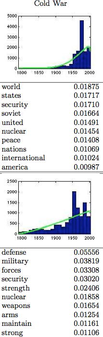
Example of two “Cold War Topics” in Topics over Time (top) and LDA (bottom) from Wang and McCallum
- Topics that don’t follow a beta distribution in their temporal pattern will be lost or split. This is where the assumption of the nature of historical change completely breaks down. Although there is sound evidence that Dirichlet distributions will apply to words across documents, there is absolutely no reason to presume that historical patterns should follow a beta distribution through time. Dirichlet distributions are convenient abstractions for topic-document distributions, but are an obviously incorrect prior for topic-year distributions. One can see this from the Ngrams data: the curves are not symmetric, but rather tend to show a brief peak followed by a long decay. I can show you a lot of camel-backed curves. A large number of words that enter the language, for example, do so in the context of wartime and so have camel-backed curves, as for the word “sniper:”

Usage of the word “sniper” in the Google Ngrams corpus (Source: Google Ngrams)
An assumption that historical changes need be continuous will end up, therefore, artificially reinforcing the already-problematic tendency of LDA to split the vocabulary of “war” (for instance) discourse into two historically conditioned ones. In analyzing newspapers, it will penalize election topics on some horizons because they peak in 2 to 4 year increments rather than smoothly building over time.
If you want to find topics that are heavily concentrated in time in a particular way, Topics over Time might be useful; but it does not seem like a good all-purpose solution to the problem of language drift.
Does that mean that modeling cannot add anything to our understanding of historical dynamics? Probably not; but it does mean that historians need to be extraordinarily cautious about interpreting the output of such models, since they will tend to privilege continuous change over discontinuous change, and unidirectional patterns over cyclical ones. (The other major temporal topic model, dynamic topic models, make their own problematic set of assumptions.) It is, perhaps, possible that someday a distributional model for change will make these models match the wide variety of historical changes that are reasonable to expect. But that ought to come out of an understanding of words or other historical units that we understand (or an understanding, at least, of the ways that we do not understand), rather than being imposed as an assumption from outside.
- [1]A few good examples of the form: Jockers, Matthew L. “The LDA Buffet Is Now Open: Or, Latent Dirichlet Allocation for English Majors.” Matthew L. Jockers, September 29, 2011. http://www.matthewjockers.net/2011/09/29/the-lda-buffet-is-now-open-or-latent-dirichlet-allocation-for-english-majors/; Underwood, Ted. “Topic Modeling Made Just Simple Enough.” The Stone and the Shell, April 7, 2012. http://tedunderwood.com/2012/04/07/topic-modeling-made-just-simple-enough/; Weingart, Scott. “Topic Modeling for Humanists: A Guided Tour.” the scottbot irregular, July 25, 2012. http://www.scottbot.net/HIAL/?p=19113; Posner, Miriam, and Andy Wallace. “Very Basic Strategies for Interpreting Results from the Topic Modeling Tool.” Miriam Posner: Blog, October 29, 2012. http://miriamposner.com/blog/?p=1335. The chapter in The Programming Historian 2 by Shawn Graham, Scott Weingart, and Ian Milligan on Topic Modeling is also very helpful.↩
- [2]David M. Blei, Andrew Ng, Michael Jordan. “Latent Dirichlet allocation,” Journal of Machine Learning Research (3) 2003 pp. 993-1022.↩
- [3]The only change to the basic constraints I made was changing the “token-regex” line so that the string “42.4,-72.1” would be parsed as a single word. Otherwise, I keep the defaults as they are.↩
- [4]There are many examples of this trend, both by historians and computer scientists. For example: Ian Milligan, “Cultural Trends in Hansard: Looking at Changes, 1994–2012”; Jonathan Goodwin, “Same Stuff, Different Graph;” Ted Underwood, “Some Results of Topic Modeling,” March 12, 2012; Mining the Dispatch from the Digital Scholarship Lab at the University of Richmond; David Hall, Daniel Jurafsky, and Christopher D. Manning. 2008. Studying the History of Ideas Using Topic Models [PDF], Proceedings of EMNLP 2008, 363–371. Paper Machines makes this widely and easily available.↩
- [5]Blei, David M., and John D. Lafferty. “Dynamic topic models.” In Proceedings of the 23rd International Conference on Machine Learning, pp. 113-120, ACM, 2006; Wang, Xuerui and Andrew McCallum. “Topics over time: a non-Markov continuous-time model of topical trends.” In Proceedings of the 12th ACM SIGKDD International Conference on Knowledge Discovery and Data Mining, pp. 424-433, ACM, 2006.↩
- [6]As an extraordinarily rough heuristic for “English,” I only included in the charts that follow topics whose first word was four or more letters long. Almost all Spanish, Latin, German and Italian topics in the corpus — of which there were several — began with a two-or-three letter word, but almost none of the English-language topics did.↩
- [7]Ramsay, Stephen. Reading Machines: Toward an Algorithmic Criticism. Topics in the Digital Humanities. Urbana: University of Illinois Press, 2011.↩
- [8]Jockers, Matthew L. Macroanalysis: Digital Methods and Literary History. University of Illinois Press, 2013.↩
- [9]Wang, Xuerui, and Andrew Mccallum. “Topics over Time: a non-Markov Continuous-time Model of Topical Trends.” In Proceedings of the 12th ACM SIGKDD International Conference on Knowledge Discovery and Data Mining, 424–433. KDD ’06. New York, NY, USA: ACM, 2006. doi:10.1145/1150402.1150450.↩