Clustering with Compression for the Historian
Chad Black
INTRODUCTION
I mentioned in my blog that I’m playing around with a variety of clustering techniques to identify patterns in legal records from the early modern Spanish Empire. In this post, I will discuss the first of my training experiments using Normalized Compression Distance (NCD). I’ll look at what NCD is, some potential problems with the method, and then the results from using NCD to analyze the Criminales Series descriptions of the Archivo Nacional del Ecuador’s (ANE) Series Guide. For what it’s worth, this is a very easy and approachable method for measuring similarity between documents and requires almost no programming chops. So, it’s perfect for me!
WHAT IS NCD?
I was inspired to look at NCD for clustering by a pair of posts by Bill Turkel (here, here) from quite a few years ago. Bill and Stéfan Sinclair also used NCD to cluster cases for the Digging Into Data Old Bailey Project. Turkel’s posts provide a nice overview of the method, which was proposed in 2005 by Rudi Cilibrasi and Paul Vitányi.[1] Essentially, Cilibrasi and Vitányi proposed measuring the distance between two strings of arbitrary length by comparing the sum of the lengths of the individually compressed files to a compressed concatenation of the two files. So, adding the compressed length of x to the compressed length of y will be longer than the compressed length of (x|y). How much longer is what is important. The formula is this, where c(x) is the length of x compressed:
NCD(x,y) = [C(x|y) - min{C(x),C(y)}] / max{C(x),C(y)
C(x|y) is the compression of the concatenated strings. Theoretically, if you concatenated and compressed two identical strings, you would get a distance of 0 because [(Cx|x) - C(x)]/C(x) would equal 0/1, or 0. As we’ll see in a bit, though, this isn’t the case and the overhead required by the various compression algorithms at our disposal make a 0 impossible, and more so for long strings depending on the method. Cilibrasi and Vitányi note that in practice, that if r is the NCD, the NCD will be 0 ≤ r ≤ 1+ ∊, where ∊ is usually around 0.1, and accounts for the implementation details of the compression algorithm. Suffice to say, though, that the closer to 0 the result is, the more similar the strings (or files in our case) are. Nonetheless, the distance between two strings, or files, or objects as measured with this formula can then be used to cluster those strings, files, or objects. One obvious advantage to the method is that it works for comparing strings of arbitrary length with one another.
Why does this work? Essentially, lossless compression suppresses redundancy in a string, while maintaining the ability to fully restore the file. Compression algorithms evolved to deal with constraints in the storage and transmission of data. It’s easy to forget in the age of the inexpensive terabyte hard drive what persistent storage once cost. In 1994, the year that the first edition of Witten, Moffat, and Bell’s Managing Gigabytes was published, hard disk storage still ran at close to $1/megabyte. That’s right, just 17 years ago that 500GB drive in your laptop would have cost $500,000. To put that into perspective, in 1980 IBM produced one of the first disk drives to break the GB barrier. The 2.52GB IBM 3380 was initially released in 5 different models, and ranged in price between $81,000 and and $142,000. For what it’s worth, the median housing price in Washington, DC in 1980 was the second highest in the country at $62,000. A hard disk that cost twice as much as the median house in DC. Obviously not a consumer product. At the per/GB rate that the 3380 sold for, your 500GB drive would have cost up to $28,174,603.17! In inflation-adjusted dollars for 2011 that would be $80.5M! An absurd comparison, to be sure. Given those constraints, efficiency in data compression made real dollars sense. Even still, despite the plunging costs of storage and growing bandwidth capacity, text and image compression remains an imperative in computer science.
As Witten, et al. define it,
Text compression … involves changing the representation of a file so that it takes less space to store or less time to transmit, yet the original file can be reconstructed exactly from the compressed representation.[2]
This is lossless compression (as opposed to lossy compression, which you may know from messing with jpegs or other image formats). There are a variety of compression methods, each of which takes a different approach to compressing text data and which are either individually or in some kind of combination behind the compression formats you’re used to–.zip, .bz2, .rar, .gz, etc. Frequently, they also have their roots in the early days of electronic data. Huffman coding was developed by an eponymous MIT graduate student in the early 1950s.
In any case, the objective of a compression method is to locate, remove, store, and recover redundancies within a text. NCD works because within a particular algorithm, the compression method is consistently imposed on the data, thus making the output comparable. What isn’t comparable, though, is mixing algorithms.
LIMITATIONS: SIZE MATTERS
Without getting too technical (mostly because I get lost once it goes too far), it’s worth noting some limitations based on which method of compression you chose when applying NCD. Shortly after Cilibrasi and Vitányi published their paper on clustering via compression, Cebrián, et al. published a piece that compared the integrity of NCD between three compressors– bzip2, gzip, and PPMZ.[3] The paper is interesting, in part, because the authors do an excellent job of explaining the mechanics of the various compressors in language that even I could understand.
I came across this paper through some google-fu because I was confused by the initial results I was getting while playing around with my Criminales Series Guide. Python has built-in support for compression and decompression using bzip2 and gzip, so that’s what I was using. I have the Criminales Series divided into decades from 1601 to 1830. My script was walking through and comparing every file in the directory to every other one, including itself. I assumed that the concatenation of two files that were identical would produce a distance measurement of 0, and was surprised to see that it wasn’t happening, and in some cases not even close. (I also hadn’t read much of anything about compression at that point!) But that wasn’t the most surprising thing. What was more surprising was that in the latter decades of my corpus, the distance measures when comparing individual decades to themselves were actually coming out very high. Or, at least they were using the gzip algorithm. For example, the decade with the largest number of cases, and thus the longest text, is 1781-1790 at about 39,000 words. Gzip returned an NCD of 0.97458 when comparing this decade to itself. What? How is that possible?
Cebrián, et al. explain how different compression methods have upper limits to the size of a block of text that they operate on before needing to break that block into new blocks. This makes little difference from the perspective of compressors doing their job, but it does have implications for clustering. The article goes into more detail, but here’s a quick and dirty overview.
bzip2
The bzip2 compressor works in three stages to compress a string: (1) a Burrows-Wheeler Transform, (2) a move-to-front transform, and (3) a statistical compressor like Huffman coding.[4] The bzip2 algorithm can perform this method on blocks of text up 900KB without needing to break the block of text into two blocks. So, for NCD purposes, this means that if a pair of files are concatenated, and the size of this pair is less than 900KB, what the bzip compressor will see is essentially a mirrored text. But, if the concatenated file is larger than 900KB, then bzip will break the concatenation into more than one block, each of which will be sent through the three stages of compression. But, these blocks will no longer be mirrors. As a result, the NCD will cease to be robust. Cebrián, et al. claim that the NCD for C(x|x) should fall in a range between 0.2 and 0.3, and anything beyond that indicates it’s not a good choice for comparing the set of documents under evaluation.
gzip
The gzip compressor uses a different method than bzip2′s block compression, one based on the Lempel-Ziv LZ77 algorithm, also known as sliding window compression. Gzip then takes the LZ77-processed string and subjects it to a statistical encoding like Huffman. It’s the first step that is important for us, though. Sliding window compression searches for redundancies by taking 32KB blocks of data, and looking ahead at the next 32KB of data. The method is much faster than bzip2′s block method. (In my experiments using python’s zlib module, code execution took about 1/2 the time as python’s bzip on default settings.) And, if the text is small, such that C(x|x) < 32KB, the NCD result is better. Cebrián, et al. find that gzip returns an NCD result in the range between 0 and 0.1. But, beyond 32KB they find that NCD rapidly grows beyond 0.9 — exactly what I saw with the large 1781-1790 file (which is 231KB).
lzma
Cebrián, et al. offer a third compressor, ppmz, as an alternative to bzip2 and gzip for files that outsize gzip and bzip2′s upper limits. Ppmz uses Prediction by Partial Match for compression, and has no upper limit on effective file size. PPM is a statistical model that uses arithmetic coding. This gets us to things I don’t really understand, and certainly can’t explain here. Suffice to say that the authors found using ppmz that C(x|x) always returned an NCD value between 0 and 0.1043. I looked around for quite a while and couldn’t find a python implementation of ppmz, but I did find another method ported to python with lzma, the compressor behind 7zip. Lzma uses a different implementation of Lempel-Ziv, utilizing a dictionary instead of a sliding window to track redundancies. What is more, the compression-dictionary can be as large as 4GB. You’d need a really, really large document to brush up against that. Though Cebrián, et al. didn’t test lzma, my experiments show the NCD of C(x|x) to be between 0.002 and 0.02! That’s awfully close to 0, and the smallest return actually came from the longest document –> 1781-1790.
THE CODE
In a way, that previous section is getting ahead of myself. I started with just zlib, and then added bzip2 and gzip, and eventually lzma for comparison sake. Let me clarify that just a bit. In python, there are two modules that use the gzip compressor:
- gzip, which is for file compression/decompression; and
- zlib, which is for compressing/decompressing strings or objects.
I was unsettled by my early zlib returns, and tried using gzip and file I/O, but got the same returns. Initially I was interested in speed, but reading Cebrián, et al. changed my mind on that. Nonetheless, I did time the functions to see which was fastest.
I based the script on Bill Turkel’s back from 2007. (Bill put all of the scripts from the days of Digital History Hacks on Github. Thanks to him for doing that!)
So, for each compressor we need a function to perform the NCD algorithm on a pair of files:
# Function to calculate the NCD of two files using lzma
def ncd_lzma(filex, filey):
    xbytes = open(filex, 'r').read()
    ybytes = open(filey, 'r').read()
    xybytes = xbytes + ybytes
    cx = lzma.compress(xbytes)
    cy = lzma.compress(ybytes)
    cxy = lzma.compress(xybytes)
    if len(cy) > len(cx):
        n = (len(cxy) - len(cx)) / float(len(cy))
    else:
        n = (len(cxy) - len (cy)) / float(len(cx))
    return n
There are small changes depending on the API of the compressor module, but this pretty much sums it up.
We need to be able to list all the files in our target directory, but ignore any dot-files like .DS_Store that creep in on OS X or source control files if you’re managing your docs with git or svn or something:
# list directory ignoring dot files
def mylistdir(directory):
    filelist = os.listdir(directory)
    return [x for x in filelist
            if not (x.startswith('.'))]
Just as an aside here, let me encourage you to put your files under source control, especially as you can accidentally damage them while developing your scripts.
We need a function to walk that list of files, and perform NCD on every possible pairing, the results of which are written to a file. For this function, we pass as arguments the file list, the results file, and the compressor function of choice:
def walkFileList(filelist, outfile, compType):
    for i in range(0, len(filelist)-1):
        print i
        for j in filelist:
            fx = pathstring+str(filelist[i])
            fy = pathstring+str(j)
            outx = str(filelist[i])
            outy = str(j)
            outfile.write(str(outx[:-4]+"  "+outy[:-4]+"  ")+str(compType(fx, fy))+"\n")
That’s all you need. I mentioned also that I wanted to compare execution time for the different compressors. That’s easy to do with a module from the python standard library called profile, which can return a bunch of information gathered from the execution of your script at runtime. To call a function with profile you simply pass the function to profile.run as a string. So, to perform NCD via lzma as described above, you just need something like this:
outfile = open('_lzma-ncd.txt', 'w')
print "Starting lzma NCD."
profile.run('walkFileList(filelist, outfile, ncd_lzma)')
print 'lzma finished.'
outfile.close()
I put the print statements in just for shits and giggles. Because we ran this through profile, after doing the NCD analysis and writing it to a file named _lzma-ncd.txt, python reports on the total number of function calls, the time per call, per function, and cumulative for the script. It’s useful for identifying bottlenecks in your code if you get to the point of optimizing. At any rate, there is no question that lzma is much slower that the others, but if you have the cpu cycles available, it may be worth the rate from a quality of data perspective. Here’s what profile tells us for the various methods:
- zlib: 7222 function calls in 16.564 CPU seconds (compressing string objects)
- gzip: 69460 function calls in 18.377 CPU seconds (compressing file objects)
- bzip: 7222 function calls in 21.129 CPU seconds
- lzma: 7222 function calls in 115.678 CPU seconds
If you expected zlib/gzip to be substantially faster than bzip, it was, until I set all of the algorithms to the highest available level of compression. I’m not sure that’s necessary or not, but it does affect the results as well as time. Note too that the gzip file method requires many more function calls, but with relatively little performance penalty.
COMPARING RESULTS
The Series Guide
A little bit more about the documents I’m trying to cluster. Beginning around 2002, the Archivo Nacional del Ecuador began to produce pdfs of their ever-growing list of Series Finders guides. The Criminales Series Guide (big pdf) was a large endeavor. The staff went through every folder in every box in the series, reorganized them, and wrote descriptions for the Series Guide. Entries in the guide are divided by box and folder (caja/expediente). A typical folder description looks like this:
Expediente: 6
Lugar: Quito
Fecha: 30 de junio de 1636
No. de folios : 5
Contenido: Querella criminal iniciada por doña Joana Requejo, mujer legítima del escribano mayor Andrés de Sevilla contra Pedro Serrano, por haber entrado a su casa y por las amenazas que profirió contra ella con el pretexto de que escondía a una persona que él buscaba.
We have the place (Quito), the date (06/30/1636), the number of pages (5), and a description. The simple description includes the name of the plaintiff, in this case Joana Requejo, and the defendant, Pedro Serrano, along with the central accusation– that Serrano had entered her house and threatened her under the pretext that she was hiding a person he was looking for. There is a wealth of information that can be extracted from that text. The Series Guides as a whole is big, constituting close to 875 pages of text and some 1.1M words. I currently have text files for the following Series Guides–> Criminales, Diezmos, Encomiendas, Esclavos, Estancos, Gobierno, Haciendas, Indígenas, Matrimoniales, Minas, Obrajes, and Oficios totaling 4.8M words. I’ll do some comparisons between the guides in the near future, and see if we can identify patterns across Series. For now, though, it’s just the Criminales striking my fancy.
The Eighteenth Century
So, what does the script give us for the 18th century? Below are the NCD results for three different compressors comparing my decade of interest, 1781-1790, with the other decades of the 18th century:
zlib:
cr1781_1790  cr1701_1710  0.982798401771
cr1781_1790  cr1711_1720  0.987881971149
cr1781_1790  cr1721_1730  0.977414695455
cr1781_1790  cr1731_1740  0.97668311167
cr1781_1790  cr1741_1750  0.975895252209
cr1781_1790  cr1751_1760  0.975088634189
cr1781_1790  cr1761_1770  0.975632632389
cr1781_1790  cr1771_1780  0.973381605357
cr1781_1790 cr1781_1790 0.974582153107
cr1781_1790  cr1791_1800  0.972256091842
cr1781_1790  cr1801_1810  0.973325329682
bzip:
cr1781_1790  cr1701_1710  0.954733848029
cr1781_1790  cr1711_1720  0.96900988758
cr1781_1790  cr1721_1730  0.929649194095
cr1781_1790  cr1731_1740  0.923066504131
cr1781_1790  cr1741_1750  0.906271163484
cr1781_1790  cr1751_1760  0.903237166463
cr1781_1790  cr1761_1770  0.902912095354
cr1781_1790  cr1771_1780  0.849356630096
cr1781_1790 cr1781_1790 0.287823378031
cr1781_1790  cr1791_1800  0.850331843424
cr1781_1790  cr1801_1810  0.850358932683
lzma:
cr1781_1790  cr1701_1710  0.965529663402
cr1781_1790  cr1711_1720  0.976516942474
cr1781_1790  cr1721_1730  0.947607790161
cr1781_1790  cr1731_1740  0.94510863447
cr1781_1790  cr1741_1750  0.931757289204
cr1781_1790  cr1751_1760  0.931757289204
cr1781_1790  cr1761_1770  0.92759202972
cr1781_1790  cr1771_1780  0.885106382979
cr1781_1790 cr1781_1790 0.0021839468648
cr1781_1790  cr1791_1800  0.880670944501
cr1781_1790  cr1801_1810  0.887110210514
First off, even just eyeballing it, you can see that the results from bzip and lzma are more reliable and follow exactly the patterns discussed by Cebrián, et al. The bzip run provides a C(x|x) of 0.288, which falls in the acceptable range. The lzma run returns a C(x|x) NCD of 0.0022, not much more needed to say there. And, as I noted above, with zlib/gzip we get 0.9745. Further, by eyeballing the results on the good runs, two relative clusters appear in the decades surrounding 1781-1790. It appears that from 1771 to 1810 that we have more similarity than in the earlier decades of the century. This accords with my expectations based on other research, and in both cases the further back from 1781 that you go, the more different the decades are on a trendline.
If we change the comparison node to, say, 1741-1750 we get the following results:
bzip:
cr1741_1750  cr1701_1710  0.888048411498
cr1741_1750  cr1711_1720  0.919398218188
cr1741_1750 cr1721_1730 0.826189275508
cr1741_1750 cr1731_1740 0.80795091612
cr1741_1750  cr1741_1750  0.277693730039
cr1741_1750 cr1751_1760 0.785168132862
cr1741_1750 cr1761_1770 0.803655071796
cr1741_1750  cr1771_1780  0.879983993015
cr1741_1750  cr1781_1790  0.906271163484
cr1741_1750  cr1791_1800  0.883904391852
cr1741_1750  cr1801_1810  0.886378259718
lzma:
cr1741_1750  cr1701_1710  0.905551014342
cr1741_1750  cr1711_1720  0.932600133759
cr1741_1750  cr1721_1730  0.862079215278
cr1741_1750 cr1731_1740 0.848926209408
cr1741_1750  cr1741_1750  0.00587055064279
cr1741_1750 cr1751_1760 0.830746598014
cr1741_1750 cr1761_1770 0.844162055066
cr1741_1750  cr1771_1780  0.90796460177
cr1741_1750  cr1781_1790  0.929573342339
cr1741_1750  cr1791_1800  0.908149721264
cr1741_1750  cr1801_1810  0.913968518045
Again, the C(x|x) show reliable data. But, this time bzip’s similarities look a fair amount different that lzma when eyeballing it. I’m interested in the decade of the 1740s in part because I expect more similarity to the latter decades than for other decades in, really, either the 18th or the 17th century. I expect this for reasons that have to do with other types of hermeneutical screwing around, to use Stephen Ramsey’s excellent phrase [PDF], that I’ve been doing with the records lately. Chief among those (and an argument for close as well as distant readings) is that I’ve been transcribing weekly jail censuses from the 1740s the past week and some patterns of familiarity have been jumping out at me. I have weekly jail counts from 1732 to 1791 inclusive, and a bunch others too. I’ve transcribed so many of these things that I have pattern expectations. And, the 1740s has jumped out at me for three reasons this week. The first is that in 1741, after a decade of rarely noting it, the notaries started to record the reason for ones detention. The second is that in 1742, and particularly under the aegis of one particular magistrate, more people started to get arrested than previous and subsequent decades. The third is that, like in the period between 1760 and 1790, those arrests were increasingly for moral offenses or for being picked up during nightly rounds of the city (the ronda). The differences are this–in the latter period women and men were arrested in almost equal numbers. There are almost no women detainees in the 1740s. And, there doesn’t seem to be an equal growth in both detentions and prosecutions in the 1740s. This makes the decade more like the 1760s than the 1780s. The results above bear that out to some extent, as distance measures show to be more like the 1760s than the 1780s.
I also had this suspicion because a few months ago I plotted occurrences of the terms concubinato (illicit co-habitation) and muerte (used in murder descriptions) from the Guide:
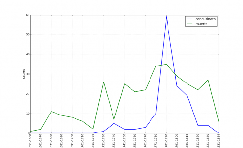
Occurrences of the terms “concubinato” and “muerte” from the Criminales Series Guide.
You should see that right at the decade of the 1740s there is a discernible, if smaller, bump for concubinato. I was reminded of this when transcribing the records.
CONCLUSION
OK, at this point, this post is probably long enough. What’s missing above is obviously visualizations of the clusters. Those visualizations are pretty interesting. For now, though, let me conclude by saying that I am impressed initially to see the clusters that emerged from this simple, if profound, technique for clustering. Given that the distinctions I’m trying to pick up are slight, I’m worried a bit about the level of precision I can expect. But, I am convinced that it’s worth sacrificing performance for either bzip or lzma implementations depending on the length of one’s documents. Unless your files are longer than 900KB, it’s probably worth just sticking with bzip.
Originally published by Chad Black on October 9, 2011. Revised March 2012.
- [1]Rudi Cilibrasi and Paul Vitányi, “Clustering by Compression,” IEEE Transactions on Information Theory 51.4 (2005): 1523-45, PDF.↩
- [2]Ian H. Witten, Alistair Moffat, and Timothy C. Bell, Managing Gigabytes: Compressing and Indexing Documents and Images, 2nd Edition (San Diego, California: Academic Press, 1999), 21.↩
- [3]Manuel Cebrián, Manuel Alfonseca, and Alfonso Ortega, “Common Pitfalls Using the Normalized Compression Distance: What to Watch Out for in A Compressor,” Communications of Information and Systems 5, no. 4 (2005): 367-384.↩
- [4]Cebrián, et al., “Common Pitfalls Using the Normalized Compression Distance,” 372.↩